ソフトウェア
OpenMebius
An integrated software for conventional 13C-MFA and isotopically nonstationary 13C-MFA (INST-13C-MFA). This work is partially supported by JST, Strategic International Collaborative Research Program, SICORP for JP-US Metabolomics.
Download OpenMebius
Operating systems
This software has been developed in MATLAB (The MathWorks, Natick,MA), which is operated only on the Windows platform.
Operating check
This software has been successfully tested on x86- and x64-based PCs running Windows 7.
Other Windows platform has no problem to operate this software, while the officially test has not been performed.
System Requirements
Operating systems: Windows platform
Software requirements: Matlab R2011a or later version
Other requirements: Matlab Statistics Toolbox, Microsoft EXCEL 2010 or later version (for reading and writing xlsx files by OpenMebius), glpkmex 2.11 from SourceForge (http://sourceforge.net/projects/glpkmex/files/glpkmex/)
Installation and configuration:
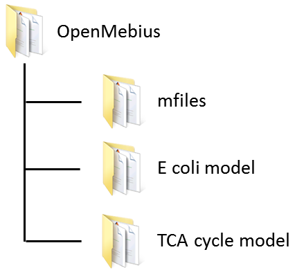
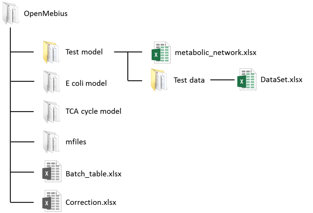
1. Extract all files in the Zip archive (OpenMebius) in your working directory.
The OpenMebius directory contains three directories, "mfiles", "E coli model" and "TCA cycle model".
2. Run MATLAB and set the "mfiles" directory as a current directory.
3. Type "Set_up_OpenMebius" in the command line to set up OpenMebius. "Correction.xlsx" and "Batch_table.xlsx" are generated in the OpenMebius directory.
4. Download the precompiled version of glpkmex 2.11 from SourceForge (http://sourceforge.net/projects/glpkmex/files/glpkmex/). The downloaded glpxmex directory is placed into the OpenMebius directory.
5. Set the "glpkmex" directory as the current directory.
6. Type "addpath(pwd)" to add the glpkmex directory to the Matlab search path.
Quick start guide
- Performance test for isotopically stationary (conventional) 13C-MFA
1. Model construction
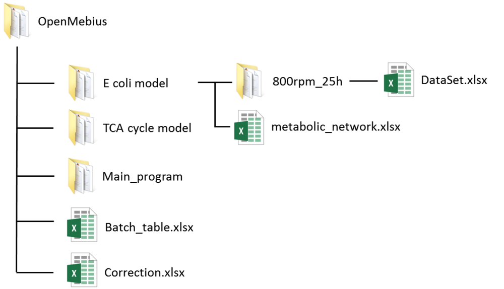
Metabolic model definition is described in "Metabolic_network.xlsx" in "Ecoli model" directory. OpenMebius is parsed the definition into MATLAB readable file format.
1-1. Run MATLAB and set "E coli model" as the current directory.
1-2. Type "[model, frag] = Modelconfig('E coli model', 'xlsx');" in the command line. ● Run time 1 sec (2.80GHz Intel Core i7 processor)
1-3. Type "[model] = ConstEMUnetwork(model, frag);" in the command line. ● Run time 2 sec (2.80GHz Intel Core i7 processor)
Five files are constructed in the directory. The stoichiometry matrix S and metabolic model M are described in "model.mat" and "CalMDV.m", respectively.
2. Experimental data inputs
All experimental data is described in "DataSet.xlsx" in "800rpm_25h" directory.
"DataSet.xlsx" describes the following information.
- "efflux" sheet
Individual flux values are given, such as production rate, biomass synthesis rate, and substrate consumption rate.
- "Substrate" sheet
Carbon numbers of each carbon source is described.
- "Abundance_list" sheet
Isotopic labeling enrichment data determined by mass spectrometry are described.
- "Components" sheet
The number of each chemical element in a mass fragment is described considering its derivatization.
- "Spectrum" sheet
Selection of labeling enrichments for data fitting.
3. Mass data processing
3-1. Open "Correction.xlsx" in OpenMebius directory using Microsoft Excel.
3-2. Input each column as below.
3-3. Save "Correction. xlsx".
3-4. Set “E coli model” as the current directory.
3-5. Type “Extract_MS” in the command line to convert raw abundances of mass spectra into the form for estimating fluxes. ● Run time 11 sec (2.80GHz Intel Core i7 processor)
The raw data is described in “DataSet.xlsx” in "800rpm_25h" directory. “DataSet.xlsx” contains all the experimental data for flux estimation, and the configuration for selecting a mass spectrum to non-linear fitting. Detailed rules of the file are described in the tutorial.
4. Metabolic flux estimation
4-1. Open “Batch_table.xlsx” using Microsoft Excel.
4-2. Input each column as below.

※ Do not describe anything in the Option column.
4-3. Set “E coli model” as the current directory.
4-4. Type “main” in the command line. ● Run time 2 min (2.80GHz Intel Core i7 processor)
4-5. The result of metabolic flux estimation is the output in “Result_all.xlsx” in the "Test data" directory.
4-6. Open “Result_all.xlsx” using Microsoft Excel. The “Flux distribution” sheet describes the summary of flux estimation as below:
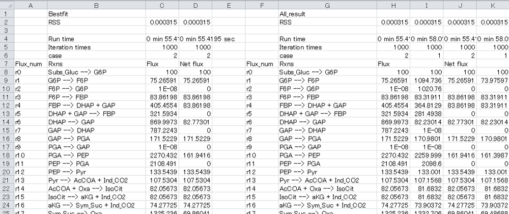
In the performance test, flux is optimized from different initial values five times.
The best-fit result and all results are described in the left block and right block, respectively.
Performance test for isotopically nonstationary (INST-13C-MFA)
1. Model construction
1-1. Run MATLAB and set “TCA cycle model” as the current directory. This directory contains “Metabolic_network.xlsx” describing the metabolic model.
1-2. Type "[model, frag] = Modelconfig('TCA cycle model', 'xlsx');" in the command line. ● Run time 1 sec (2.80GHz Intel Core i7 processor)
1-3. Type "[model] = ConstEMUnetwork(model, frag);" in the command line. ● Run time 2 sec (2.80GHz Intel Core i7 processor)
Stoichiometry matrix S and metabolic model M are automatically constructed in the directory.
2. Prepare input data set
2-1. Open "Correction.xlsx" in OpenMebius directory using Microsoft Excel.
2-2. Input each column as below.
2-3. Save "Correction. xlsx".
2-4. Set “TCA cycle model” as the current directory.
2-5. Type “Extract_MS_inst” in the command line to convert raw abundances of mass spectra into the form for estimating fluxes. ● Run time 30 sec (2.80GHz Intel Core i7 processor)
The raw data is described in “DataSet.xlsx” in the "Artificial data" directory. “DataSet.xlsx” contains all the experimental data for flux estimation, and the configuration for selecting the mass spectrum to non-linear fitting. Detailed rules of the file are described in the tutorial.
3. Metabolic flux estimation
3-1. Open “Batch_table.xlsx” in the OpenMebius directory.
3-2. Input each column as follows:

※ Do not describe anything in the Option column.
3-3. Set “TCA cycle model” as the current directory.
3-4. Type “main” in the command line. ● Run time 15 min (2.80GHz Intel Core i7 processor)
3-5. The result of metabolic flux estimation is the output "Result_case1.xlsx" in the "Artificial data" directory. The accurate estimate is indicated as below.
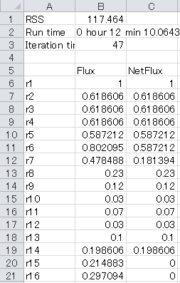
The result depends on the initial values of the fluxes and the estimate value is sometimes wrong. If this is the case, please retry with a new estimate of metabolic flux.
Tutorial
Model construction:
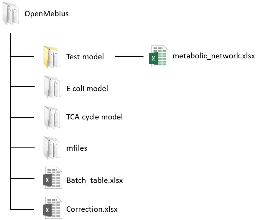
1. Create a model directory (ex. E coli model and TCA cycle model) in the OpenMebius directory.
2. Set the model directory as the current directory by MATLAB.
3. Type "MakeModelconfig" in the command line.
The model configuration file "Metabolic_network.xlsx" is automatically generated in the model directory.
Example:
If you create "Test model", the directory structure is as shown below:
4. Open "Metabolic_network.xlsx" in Microsoft Excel, and describe the configuration of the metabolic model on the three worksheets"mass_balance", "Substrate", and "MSReac".
- "mass_balance" sheet
The metabolic pathway and carbon transition networks are described in 6 columns in the "mass_balance" sheet.
a. FluxID column: Unique reaction names such as IDs or gene symbols.
b. Rxns column: Equations of metabolic reactions. Identifiers of metabolites must follow the description rules below.
Table: Description rules for metabolite identifiers in the Rxns column
Tag | DESCRIPTION |
Subs_ | Prefix for carbon sources such as glucose and glutamine |
Sym_ | Prefix for metabolites with symmetric structures such as succinate and fumarate |
Ind_CO2 | Reserved word for CO2. OpenMebius determines the isotopic labeling enrichment of CO2 as an independent variable. |
Ind_THF | Reserved word for tetrahydrofolic acid (THF) used in the alanine and glycine biosynthetic pathways. OpenMebius determines the isotopic labeling enrichment of THF as an independent variable. |
[ ] | Metabolic identifiers in square brackets are considered to be outside the metabolic systems (such as products excreted to the medium and those that are used for biomass formation) |
[Caution]
・Identifiers of metabolites have to be more than four letters in length.
・The numbers of reactants and products must be less than two.
・When two identical metabolites are produced by the reaction such as "A --> 2 B", please describe the reaction as "A --> B + C" and "C --> B" using the pseudo metabolite "C".
・Reactions for biomass synthesis and product excretion have to be described under the central metabolism reactions.
c. NetFlux column: combination of reversible reactions
A combination of reversible reactions is input as the same number on this column. The numbers are used from one without missing any numbers to the total combination of reversible reactions. An irreversible reaction is input as zero.
d. Carbon transitions column: Mapping of carbon atom transitions among reactants and products.
For instance, the transition “ABCDEF --> CBA + DEF” of the reaction “FBP --> DHAP + GAP” indicates that the C1 carbon in fructose-1,6-bisphosphate (FBP) (A) is transferred to the C3 carbon in dihydeoxyacetone phosphate (DHAP).
e. Option column: Select free flux
"A" is denoted if an efflux reaction should be considered as an independent variable.
- "Substrate" sheet
The carbon numbers of each carbon source are described in the “Substrate” sheet.
a. Name column: Identifiers (names) of carbon sources that include the prefix "Subs_".
b. C_number column: Carbon numbers of each carbon source
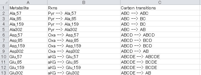
- "MSReac" sheet
The composition of each fragment of metabolite whose isotopic labeling enrichment is measured by mass spectrometry is described in the “MSReac sheet”
For example, the row “Ala_85, Pyr --> Ala_85, ABC --> BC” indicates that carbons in the [M-85]+ fragment of alanine are derived from the C2 and C3 carbons of pyruvate.
a. Metabolite column: Unique identifiers for each mass fragment of metabolites.
b. Rxns column: Composition of each metabolite
Table Descriptions of tag used for “Rxns” column
Tag | DESCRIPTION |
Sym_ | Prefix for metabolites with symmetry structure such as succinate and fumalate |
[Caution]
・Identifiers of metabolites should be more than four letters in length.
・Distinct naming rules are employed for Conventional 13C-MFA and isotopically nonstationary 13C-MFA.
Conventional 13C-MFA
・Unlimited numbers of reactants and only one product are permitted per reaction.
・Redundant reactants such as “Pyr + Pyr --> Val_85” are permitted.
In the case of INST-13C-MFA
・One reactant and one product per reaction are allowed.
c. Carbon transitions column: Identical rule as in the “Mass_balance” sheet.
5. Type "[model, frag] = Modelconfig(modelname, 'xlsx');" in the command line in the model directory.
The "modelname" is the model directory name.
6. Type "[model] = ConstEMUnetwork(model, frag);" in the command line in the model directory.
The stoichiometry matrix S and the metabolic model M are automatically constructed in the directory.
Prepare the experimental data:
- Set directory to use metabolic flux estimation
- Type "MakeDataSet" in the command line in the model directory.
- Type a data name following the message:
Please input data name >
Example:
If you create "Test model" and obtain experimental data named "Test data", the "Test data" directory should be created as follows.
4. Open "DataSet.xlsx" using Microsoft Excel and describe following information.
- "efflux" sheet
a. FluxID column: Unique identifiers of efflux reactions (ex. production rate, biomass synthesis) and carbon source consumption rate corresponding to that in the “Mass_balance” sheet.
b. Flux column: Flux values of each efflux reaction. Whereas the flux values are permitted in proper units (such as mmol/gDCW/h) in conventional 13C-MFA , flux values are determined as "μmol/gDCW/sec" in isotopic nonstationary 13C-MFA. The efflux values are determined by analyses of product levels in the culture medium.
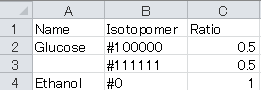
- "Substrate" sheet
Isotopic labeling patterns of carbon sources are described in "Substrate" sheet.
a. Name column: Identifiers of carbon source are identical with those in the “Substrate” sheet in Metabolic_network.xlsx. Please discard the prefix ’Subs_’ from the carbon source name.
b. Isotopomer column: Patterns of isotope labeling are described using “1” (13C labeled) and “0” (non-labeled) such as #100000 for [1-13C] glucose.
c. Ratio column: Ratios of each isotopomer in the carbon source.
For the case of a labeling experiment using a mixture of 13C labeled glucose ([1-13C]glucose:[U-13C]glucose = 50:50) and non-labeled ethanol as the carbon source, the “Substrate” sheet should be configured as follows:
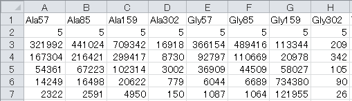
- "Abundance_list" sheet
Isotopic labeling enrichment data determined by mass spectrometry are described in the "Abundance_list" sheet. Each column corresponds to one mass fragment of measured metabolites.
First row: Name of fragment
Second row: Total number of measurable mass isotopomer in each mass fragment
Bottom rows: Raw abundance of each mass isotopomer described in order from M0
Blank cells should be filled with zero.
In the case of INST-13C MFA, multiple “Abundance_list” sheets are prepared for each time point. Sheet numbers such as "Abundance_list1", "Abundance_list2", and "Abundance_list3" represent the order of time points.
- "Components" sheet
The number of each chemical element in a mass fragment is described, taking into consideration the derivatization.
Table: Descriptions of tags used for the “Rxns” column
| Column | DESCRIPTION |
Name | Unique identifiers for each mass fragment corresponding to the MSReac sheet in Metabolic_network.xlsx |
C | Number of carbon atoms other than those in the carbon skeleton |
H | Number of hydrogen atoms |
O | Number of oxygen atoms |
S | Number of sulfur atoms |
Si | Number of silica atoms |
Carbon Skeleton | Number of carbon atoms in carbon skeleton |
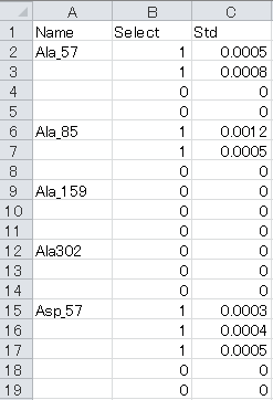
- "Spectrum" sheet
a. Name column: Unique identifiers of each metabolite or mass fragment corresponding to the “Abundance_list” sheet
b. Select column: Selection of labeling enrichment data for MFA as “1” (used) or “0” (ignored).
c. Std column: Standard deviations of isotopic labeling enrichment data. Please use “1” if unavailable.
< Only isotopically nonstationary>
- "Initial_pool" sheet
Pool size of each metabolite (μmol/g-drycell)
- "Time_course" sheet
List of sampling times (seconds)
Mass data processing:
Summary
a. Correction of naturally occurring isotopes
Effects derived from naturally occurring isotopes should be removed from row mass spectra data for the precise determination of isotope labeling enrichment of 13C derived from the carbon source. OpenMebius has this function using a correction matrix.
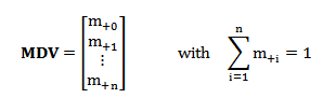
b. Normalization
Isotopic labeling enrichment shows the relative abundance of various isotopic patterns, which is described by a mass distribution vector (MDV) assigning the ratio of the mass fraction to the element.
Procedure
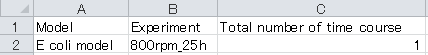
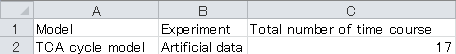
1. Open “Correction.xlsx” file in root directory using Microsoft Excel to configure the following information in the Correction sheet.
a. Model column: Model directory name
b. Experiment column: Experimental directory name
c. Total number of time courses: Total number of time courses is provided. In the case of conventional 13C-MFA, the value is "1".
2. Set the model directory as the current directory for MATLAB
3. Type “Extract_MS” in the command line for performing conventional 13C-MFA and type “Extract_MS_inst” for performing isotopically nonstationary 13C-MFA.
Metabolic flux estimation:
1. Open "Batch_table.xlsx" in the root directory using Microsoft Excel to prepare information for a metabolic flux estimation.
a. Model column: Name of model directory for flux estimation
b. Experiment column: Name of experiment directory for flux estimation.
c. Iteration time column: Maximal number of iterations in an optimization using the Levenberg-Marquardt algorithm.
d. Number of trials column: Number of flux estimation trials
e. THF column: Existence of THF in the metabolite model
f. Isotopic labeling column: Choose conventional 13C-MFA or INST-13C-MFA.
g. Option column: Please describe "Grid" to estimate 95% confidence intervals using the grid search algorithm
Estimation of confidence interval:
Summary
Confidence intervals of flux estimations are determined by OpenMebius using the grid search method. The metabolic flux of reaction r is fixed to vbest,r + d and the objective function is re-optimized. Here, vbest,r is the best fitted metabolic flux of reaction r and d is the perturbation level. The procedure is iterated with increased or decreased d. The range of fixed metabolic flux whose sum of squared residuals is less than the threshold level is the confidence interval. The threshold level is determined by
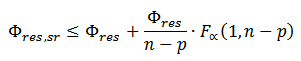
Where Φres, sr is the minimized squared sum of residuals with one fixed flux, Φres is the original minimized squared sum of residuals, n is the number of independent data points used in the fitting, p is the degrees of freedom in the original flux fit, F is the F-distribution, and α is the confidence level.
Procedure
1. Describe “Grid” in the “Option” column in “Batch_table.xlsx”
2. Add the “Grid” sheet to “DataSet.xlsx”
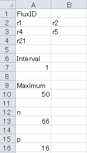
3. Configure the “Grid” sheet.
For example, to perform a grid search for one irreversible (r21) and two reversible (r1+r2, r4+r5) reactions using a maximum search width of 50 with a grid step of 1 in the fitting with 16 degrees of freedom and 66 independent measures, the “Grid” sheet should be configured as below. Please do not indicate "fixed" reaction ids (reactions listed in "Efflux" sheet of DataSet.xlsx) in FluxID.